Remote Sensing

Instructor

Dr. Zubairul Islam
Office location Block 105,
Room – 36
Adigrat university
Telephone 0967490505
Email zubairul@gmail.com

Course Description

This course introduces the theory and techniques of remote sensing and their application in geographic variables. It emphasizes on computer algorithms and digital image processing techniques. It gives basic concepts and definitions of remote sensing, and its applications. It deals with the description of electromagnetic energy and their interaction to the atmosphere and the surface of the earth. This course also explains the platforms in aerial and space borne imagery, Visual image interpretation, image enhancement, image classification methods and the technology of global positioning system.

Course Objective

Up on the successful completion of the course, students will be able to:

Explore concepts, and historical development of Remote sensing

Identify the principles of how remote sensing images are acquired

Understand how Electromagnetic radiation interacts with the Earth & atmosphere

Interoperate and extract usable information from remotely sensed images using remote sensing image processing computer systems

Explore the potential applications of remote sensing images in solving real world geographic problems.

Examine the advantages of using remote sensing image data in solving real world geographic problems

Identify the characteristics of different types of remote sensing images and their respective application

Applications of GPS

Course Content

CHAPTER 1 – INTRODUCTION

1.1. Definition of Remote Sensing

“Remote sensing is the science (and to some extent, art) of acquiring information about the Earth’s surface without actually being in contact with it. This is done by sensing and recording reflected or emitted energy and processing, analyzing, and applying that information.”

1.2. Elements of Remote Sensing

1.2.1 Energy Source or Illumination (A) –The First requirement for remote sensing is to have an energy source which illuminates or provides electromagnetic energy to the target of interest.
1.2.2. Radiation and the Atmosphere (B) – As the energy travels from its source to the target, it will come in contact with and interact with the atmosphere it passes through. This interaction may take place a second time as the energy travels from the target to the
1.2.3. Interaction with the Target (C) – once the energy makes its way to the target through the atmosphere, it interacts with the target depending on the properties of both the target and the radiation.
1.2.4. Recording of Energy by the Sensor (D) – after the energy has been scattered by, or emitted from the target, we require a sensor (remote – not in contact with the target) to collect and record the electromagnetic radiation.
1.2.5. Transmission, Reception, and Processing (E) – the energy recorded by the sensor has to be transmitted, often in electronic form, to a receiving and processing station where the data are processed into an image (hardcopy and/or digital).
1.2.6. Interpretation and Analysis (F) – the processed image is interpreted, visually and/or digitally or electronically, to extract information about the target which was illuminated.
1.2.7. Application (G) – the final element of the remote sensing process is achieved when we apply the information we have been able to extract from the imagery about the target in order to better understand it, reveal some new information, or assist in solving a particular problem.

1.3 Advantages of Remote Sensing

Enables to observe a broad area at a time

Enables to observe the area for a long period –Repeat pass observation (Time series data, Change detection)
Enables to know the condition without visiting the area
Enables to know invisible information – Sensors for various electromagnetic spectrum (Infrared, microwave)

Current major applications of remote sensing may as following:

Geology: In geology, for instance, remote sensing can be applied to analyze and map large, remote areas. Remote sensing interpretation also makes it easy for geologists in this case to identify an area’s rock types, geomorphology, and changes from natural events such as a flood or landslide.
Forestry: Satellite imagery is used to identify and map: – • The species of native and exotic forest trees. • The effects of major diseases or adverse change in environmental conditions. • The geographic extent of forests. etc
Change detection: Satellite imagery is not always able to provide exact details about the species or age of vegetation. However, the imagery provides a very good means of measuring significant change in vegetation cover, whether it is through clearing, wildfire damage or environmental stress. The most common form of environmental stress is water deficiency.
Oceanography: Remote sensing is applied to oceanography studies. Remote sensing is used, for example, to measure sea surface temperature and to monitor marine habitats.
Meteorology: Remote sensing is an effective method for mapping cloud type and extent, and cloud top temperature.

CHAPTER 2 – ELECTROMAGNETIC RADIATION AND SPECTRUM

2.1. Electromagnetic radiation

The first requirement for remote sensing is to have an energy source to illuminate the target (unless the sensed energy is being emitted by the target). This energy is in the form of electromagnetic radiation.
Two characteristics of electromagnetic radiation are particularly important for understanding remote sensing.
These are the wavelength and frequency.
The wavelength is the length of one wave cycle, which can be measured as the distance between successive wave crests.
Wavelength is usually represented by the Greek letter lambda (λ). Wavelength is measured in metres (m) or some factor of metres such as nanometres (nm, 10-9 metres), micrometres (μm, 10-6 metres) (μm, 10-6 metres) or centimetres (cm, 10-2 metres).
Frequency refers to the number of cycles of a wave passing a fixed point per unit of time.
Wavelength and frequency are inversely related to each other. The shorter the wavelength, the higher the frequency.

The electromagnetic (EM) spectrum

The electromagnetic (EM) spectrum is the continuous range of electromagnetic radiation, extending from gamma rays (highest frequency & shortest wavelength) to radio waves (lowest frequency & longest wavelength) and including visible light.
The EM spectrum can be divided into seven different regions —gamma rays, X-rays, ultraviolet, visible light, infrared, microwaves and radio waves.
Remote sensing involves the measurement of energy in many parts of the electromagnetic (EM) spectrum. The major regions of interest in satellite sensing are visible light, reflected and emitted infrared, and the microwave regions. The measurement of this radiation takes place in what are known as spectral bands. A spectral band is defined as a discrete interval of the EM spectrum.
For example the wavelength range of 0.4μm to 0.5μm (μm = micrometers or 10-6m) is one spectral band.
Satellite sensors have been designed to measure responses within particular spectral bands to enable the discrimination of the major Earth surface materials. Scientists will choose a particular spectral band for data collection depending on what they wish to examine.
The design of satellite sensors is based on the absorption characteristics of Earth surface materials across all the measurable parts in the EM spectrum.
Visible Spectrum
The light which our eyes – our “remote sensors” – can detec​t is part of the visible spectrum.
It is important to recognize how small the visible portion is relative to the rest of the spectrum.
There is a lot of radiation around us which is invisible to our eyes, but can be detected by other remote sensing instruments and used to our advantage.
It is important to note that this is the only portion of the EM spectrum we can associate with the concept of colours.
Blue, green, and red are the primary colors or wavelengths of the visible spectrum.
They are defined as such because no single primary color can be created from the other two, but all other colors can be formed by combining blue, green, and red in various proportions.
Although we see sunlight as a uniform or homogeneous color, it is actually composed of various wavelengths of radiation in primarily the ultraviolet, visible and infrared portions of the spectrum.
The visible portion of this radiation can be shown in its component colors when sunlight is passed through a prism.
Infrared (IR) Region
The IR Region covers the wavelength range from approximately 0.7 μm to 100 μm – more than 100 times aswide as the visible portion!
The IR region can be divided into two categories based on their radiation properties – the reflected IR, and the emitted or thermal IR.
Reflected and Thermal IR
Radiation in the reflected IR region is used for remote sensing purposes in ways very similar to radiation in the visible portion. The reflected IR covers wavelengths from approximately 0.7 μm to 3.0 μm.
The thermal IR region is quite different than the visible and reflected IR portions, as this energy is essentially the radiation that is emitted from the Earth’s surface in the form of heat. The thermal IR covers wavelengths from approximately 3.0 μm to 100 μm.
Microwave Region
The portion of the spectrum of more recent interest to remote sensing is the microwave region from about 1 mm to 1 m.
This covers the longest wavelengths used for remote sensing.
The shorter wavelengths have properties similar to the thermal infrared region while the longer wavelengths approach the wavelengths used for radio broadcasts.

2.2. Energy Interactions with the Atmosphere

Before radiation used for remote sensing reaches the Earth’s surface it has to travel through some distance of the Earth’s atmosphere. Particles and gases in the atmosphere can affect the incoming light and radiation.
These effects are caused by the mechanisms of Scattering and absorption.

Scattering

Scattering occurs when particles or large gas molecules present in the atmosphere interact with and cause the electromagnetic radiation to be redirected from its original path. How much scattering takes place depends on several factors including the wavelength of the radiation, the abundance of particles or gases, and the distance the radiation travels through the atmosphere.
There are three (3) types of scattering which take place.
Rayleigh scattering occurs when particles are very small compared to the wavelength of the radiation. These could be particles such as small specks of dust or nitrogen and oxygen molecules. Rayleigh scattering causes shorter wavelengths of energy to be scattered much more than longer wavelengths. Rayleigh scattering is the dominant scattering mechanism in the upper atmosphere. The fact that the sky appears “blue” during the day is because of this Phenomenon. Red color at sunrise and sunset is also because of this phenomena.
Mie scattering occurs when the particles are just about the same size as the wavelength of the radiation. Dust, pollen, smoke and water vapour are common causes of Mie scattering which tends to affect longer wavelengths than those affected by Rayleigh scattering. Mie scattering occurs mostly in the lower portions of the atmosphere where larger particles are more abundant, and dominates when cloud conditions are overcast.
The final scattering mechanism of importance is called non-selective scattering. This occurs when the particles are much larger than the wavelength of the radiation. Water droplets and large dust particles can cause this type of scattering. 
Non-selective scattering gets its name from the fact that all wavelengths are scattered about equally.
This type of scattering causes fog and clouds to appear white to our eyes because blue, green, and red light are all scattered in approximately equal quantities (blue+green+red light = white light).

Absorption
Absorption is the other main mechanism at work when electromagnetic radiation interacts with the atmosphere. In contrast to scattering, this phenomenon causes molecules in the atmosphere to absorb energy at various wavelengths. Ozone, carbon dioxide, and water vapour are the three main atmospheric constituents which absorb radiation.
Ozone serves to absorb the harmful (to most living things) ultraviolet radiation from the sun. Without this protective layer in the atmosphere, our skin would burn when exposed to sunlight.
Carbon dioxide referred to as a greenhouse gas. This is because it tends to absorb radiation strongly in the far-infrared portion of the spectrum – that are associated with thermal heating – which serves to trap this heat inside the atmosphere. Water vapour in the atmosphere absorbs much of the incoming longwave infrared and short wave microwave radiation (between 22μm and 1m). The presence of water vapour in the lower atmosphere varies greatly from location to location and at different times of the year. For example, the air mass above a desert would have very little water vapour to absorb energy, while the tropics would have high concentrations of water vapour (i.e. high humidity).
Because these gases absorb electromagnetic energy in very specific regions of the spectrum, they influence where (in the spectrum) we can “look” for remote sensing purposes. Those areas of the spectrum which are not severely influenced by atmospheric absorption and thus, are useful to remote sensors, are called atmospheric windows.

Atmospheric windows

By comparing the characteristics of the two most common energy/radiation sources (the sun and the earth) with the atmospheric windows available to us, we can define those wavelengths that we can use most effectively for remote sensing. The visible portion of the spectrum, to which our eyes are most sensitive, corresponds to both an atmospheric window and the peak energy level of the sun. Note also that heat energy emitted by the Earth corresponds to a window around 10 μm in the thermal IR portion of the spectrum, while the large window at wavelengths beyond 1 mm is associated with the microwave region.

2.3 Energy interaction with the earth’s surface

Radiation that is not absorbed or scattered in the atmosphere can reach and interact with the Earth’s surface.
There are three (3) forms of interaction that can take place when energy strikes, or is incident (I) upon the surface.
These are: absorption (A); transmission (T); and reflection (R).
The total incident energy will interact with the surface in one or more of these three ways. The proportions of each will depend on the wavelength of the energy and the material and condition of the feature.
Absorption (A) occurs when radiation (energy) is absorbed into the target while transmission (T) occurs when radiation passes through a target. Reflection (R) occurs when radiation “bounces” off the target and is redirected. In remote sensing, we are most interested in measuring the radiation reflected from targets. We refer to two types of reflection, which represent the two extreme ends of the way in which energy is reflected from a target: specular reflection and diffuse reflection.
Let’s take a look at a couple of examples of targets at the Earth’s surface and how energy at the visible and infrared wavelengths interacts with them.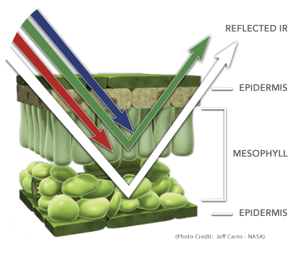

 

Leaves: A chemical compound in leaves called chlorophyll strongly absorbs radiation in the red and blue wavelengths but reflects green wavelengths. Leaves appear greenest to us in the summer, when chlorophyll content is at its maximum. In autumn, there is less chlorophyll in the leaves, so there is less absorption and proportionately more reflection of the red wavelengths, making the leaves appear red or yellow (yellow is a combination of red and green wavelengths). The internal structure of healthy leaves act as excellent diffuse reflectors of near-infrared wavelengths. If our eyes were sensitive to near-infrared, trees would appear extremely bright to us at these wavelengths. In fact, measuring and monitoring the near-IR reflectance is one way that scientists can determine how healthy (or unhealthy) vegetation may be.

 

Water: Longer wavelength visible and near infrared radiation is absorbed more by water than shorter visible wavelengths. Thus water typically looks blue or blue-green due to stronger reflectance at these shorter wavelengths, and darker if viewed at red or near infrared wavelengths. If there is suspended sediment present in the upper layers of the water body, then this will allow better reflectivity and a brighter appearance of the water. The apparent colour of the water will show a slight shift to longer wavelengths. Suspended sediment (S) can be easily confused with shallow (but clear) water, since these two phenomena appear very similar. Chlorophyll in algae absorbs more of the blue wavelengths and reflects the green, making the water appear more green in colour when algae is present. The topography of the water surface (rough, smooth, floating materials, etc.) can also lead to complications for water-related interpretation due to potential problems of specular reflection and other influences on colour and brightness.

CHAPTER 3 – SATELLITE & IMAGES CHARACTERISTICS

3.1. Satellite Sensors and platforms

3.1.1 Satellite Sensors and platforms
A sensor is a device that measures and records electromagnetic energy.
Sensors can be divided into two groups.
1. Passive sensors depend on an external source of energy, usually the sun. Most of the satellite sensors are passive.
2. Active sensors have their own source of energy, an example would be a radar gun. These sensors send out a signal and measure the amount reflected back. Active sensors are more controlled because they do not depend upon varying illumination conditions
3.1.2 Satellite Characteristics: Orbits and Swaths
Orbits
Satellites have several unique characteristics that make them particularly useful for remote sensing of the Earth’s surface. The path followed by a satellite is referred to as its orbit. Satellite orbits are matched to the capability and objective of the sensor(s) they carry. Orbit selection can vary in terms of altitude (their height above the Earth’s surface) and their orientation and rotation relative to the Earth.
Geostationary orbits
Satellites at very high altitudes, which view the same portion of the Earth’s surface at all times have geostationary orbits. These geostationary satellites revolve at speeds that match the rotation of the Earth, so they seem stationary, relative to the Earth’s surface. This allows the satellites to observe and collect information continuously over specific areas. Weather and communications satellites commonly have these types of orbits. Due to their high altitude, some geostationary weather satellites can monitor weather and cloud patterns covering an entire hemisphere of the Earth.
Sun-synchronous
Many remote sensing platforms are designed to follow an orbit (basically north-south) which, in conjunction with the Earth’s rotation (west-east), allows them to cover most of the Earth’s surface over a certain period of time. These are near-polar orbits, so named for the inclination of the orbit relative to a line running between the North and South poles. These satellite orbits are known as sun-synchronous.
Swath
As a satellite revolves around the Earth, the sensor “sees” a certain portion of the Earth’s surface. The area imaged on the surface is referred to as the swath.
Imaging swaths for space borne sensors generally vary between tens and hundreds of kilometres wide. As the satellite orbits the Earth from pole to pole, its east-west position wouldn’t change if the Earth didn’t rotate.
However, as seen from the Earth, it seems that the satellite is shifting westward because the Earth is rotating (from west to east) beneath it. This apparent movement allows the satellite swath to cover a new area with each consecutive pass. The satellite’s orbit and the rotation of the Earthwork together to allow complete coverage of the Earth’s surface, after it has completed one complete cycle of orbits.

3.2. Satellite Image data characteristics

Image data characteristics can be explained under three categories as follows:
1. The spatial resolution,
2. Spectral resolution
3. Radiometric resolution
4. Temporal resolution
3.2.1- Spatial Resolution, Pixel size and scale
The detail discernible in an image is dependent on the spatial resolution of the sensor and refers to the size of the smallest possible feature that can be detected. Spatial resolution of passive sensors (we will look at the special case of active microwave sensors later) depends primarily on their Instantaneous Field of View (IFOV).
The IFOV is the angular cone of visibility of the sensor (A) and determines the area on the Earth’s surface which is “seen” from a given altitude at one particular moment in time (B). The size of the area viewed is determined by multiplying the IFOV by the distance from the ground to the sensor (C). This area on the ground is called the resolution cell and determines a sensor’s maximum spatial resolution.
For a homogeneous feature to be detected, its size generally has to be equal to or larger than the resolution cell. If the feature is smaller than this, it may not be detectable as the average brightness of all features in that resolution cell will be recorded. However, smaller features may sometimes be detectable if their reflectance dominates within a particular resolution cell allowing sub-pixel or resolution cell detection.
PIXEL
Most remote sensing images are composed of a matrix of picture elements, or pixels, which are the smallest units of an image. Image pixels are normally square and represent a certain area on an image. It is important to distinguish between pixel size and spatial resolution – they are not interchangeable. If a sensor has a spatial resolution of 20 metres and an image from that sensor is displayed at full resolution, each pixel represents an area of 20m x 20m on the ground. In this case the pixel size and resolution are the same. However, it is possible to display an image with a pixel size different than the resolution.
Images where only large features are visible are said to have coarse or low resolution. In fine or high resolution images, small objects can be detected. Military sensors for example, are designed to view as much detail as possible, and therefore have very fine resolution. Commercial satellites provide imagery with resolutions varying from a few metres to several kilometers. Generally speaking, the finer the resolution, the less total ground area can be seen.

3.2.2- Spectral Resolution
Different classes of features and details in an image can often be distinguished by comparing their responses over distinct wavelength ranges. Broad classes, such as water and vegetation, can usually be separated using very broad wavelength ranges – the visible and near infrared other more specific classes, such as different rock types, may not be easily distinguishable using either of these broad wavelength ranges and would require comparison at much finer wavelength ranges to separate them. Thus, we would require a sensor with higher spectral resolution. Spectral resolution describes the ability of a sensor to define fine wavelength intervals. The finer the spectral resolution, the narrower the wavelength ranges for a particular channel or band.
Black and white film records wavelengths extending over much, or all of the visible portion of the electromagnetic spectrum. Its spectral resolution is fairly coarse, as the various wavelengths of the visible spectrum are not individually distinguished and the overall reflectance in the entire visible portion is recorded.
Color film is also sensitive to the reflected energy over the visible portion of the spectrum, but has higher spectral resolution, as it is individually sensitive to the reflected energy at the blue, green, and red wavelengths of the spectrum. Thus, it can represent features of various colors based on their reflectance in each of these distinct wavelength ranges.
Many remote sensing systems record energy over several separate wavelength ranges at various spectral resolutions. These are referred to as multi-spectral sensors and will be described in some detail in following sections. Advanced multi-spectral sensors called hyperspectralsensors, detect hundreds of very narrow spectral bands throughout the visible, near-infrared, and mid-infrared portions of the electromagnetic spectrum. Their very high spectral resolution facilitates fine discrimination between different targets based on their spectral response in each of the narrow bands.

3.2.3- Radiometric Resolution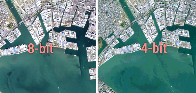
The radiometric characteristics describe the actual information content in an image. Every time an image is acquired on film or by a sensor, its sensitivity to the magnitude of the electromagnetic energy determines the radiometric resolution. The radiometric resolution of an imaging system describes its ability to discriminate very slight differences in energy the finer the radiometric resolution of a sensor, the more sensitive it is to detecting small differences in reflected or emitted energy.
Imagery data are represented by positive digital numbers which vary from 0 to (one less than) a selected power of 2. This range corresponds to the number of bits used for coding numbers in binary format. Each bit records an exponent of power 2 (e.g. 1 bit=2 1=2). The maximum number of brightness levels available depends on the number of bits used in representing the energy recorded.
Thus, if a sensor used 8 bits to record the data, there would be 28=256 digital values available, ranging from 0 to 255.
However, if only 4 bits were used, then only 24=16 values ranging from 0 to 15 would be available. Thus, the radiometric resolution would be much less.
Image data are generally displayed in a range of grey tones, with black representing a digital number of 0 and white representing the maximum value (for example, 255 in 8-bit data). By comparing a 2-bit image with an 8-bit image, we can see that there is a large difference in the level of detail discernible depending on their radiometric resolutions.
3.2.4- Temporal Resolution
In addition to spatial, spectral, and radiometric resolution, the concept of temporal resolution is also important to consider in a remote sensing system.
The revisit period of a satellite sensor is usually several days. Therefore the absolute temporal resolution of a remote sensing system to image the exact same area at the same viewing angle a second time is equal to this period.
The time factor in imaging is important when:
• Persistent clouds offer limited clear views of the Earth’s surface (often in the tropics)
• Short-lived phenomena (floods, oil slicks, etc.) need to be imaged
• Multi-temporal comparisons are required (e.g. the spread of a forest disease from one year to the next)
• The changing appearance of a feature over time can be used to distinguish it from near-similar features (wheat / maize)

3.3. Image Specifications of Multispectral Satellite Sensors

Landsat

The Landsat 8 satellite orbits the the Earth in a sun-synchronous, near-polar orbit, at an altitude of 705 km (438 mi), inclined at 98.2 degrees, and circles the Earth every 99 minutes.  The satellite has a 16-day repeat cycle with an equatorial crossing time: 10:00 a.m. +/- 15 minutes.  

Landsat 8 data are acquired on the Worldwide Reference System-2 (WRS-2) path/row system, with swath overlap (or sidelap) varying from 7 percent at the Equator to a maximum of approximately 85 percent at extreme latitudes. The scene size is 170 km x 185 km (106 mi x 115 mi). 

Data products created from over 1.3 million Landsat 8 OLI/TIRS scenes are available to download from EarthExplorer, GloVis, and the LandsatLook Viewer. 

Landsat 8 Instruments

Operational Land Imager (OLI)  –  Built by Ball Aerospace & Technologies Corporation

• Nine spectral bands, including a pan band:
  • Band 1 Visible  – Spectral resolution -(0.43 – 0.45 µm),  Spatial resolution – 30 m
  • Band 2 Visible – Spectral resolution -(0.450 – 0.51 µm),  Spatial resolution -30 m
  • Band 3 Visible – Spectral resolution -(0.53 – 0.59 µm),  Spatial resolution -30 m
  • Band 4 Red – Spectral resolution -(0.64 – 0.67 µm),  Spatial resolution -30 m
  • Band 5 Near– Spectral resolution -Infrared (0.85 – 0.88 µm),  Spatial resolution -30 m
  • Band 6 SWIR 1- Spectral resolution -(1.57 – 1.65 µm),  Spatial resolution – 30 m
  • Band 7 SWIR 2 – Spectral resolution -(2.11 – 2.29 µm),  Spatial resolution – 30 m
  • Band 8 Panchromatic (PAN) – Spectral resolution -(0.50 – 0.68 µm),  Spatial resolution – 15 m
  • Band 9 Cirrus – Spectral resolution -(1.36 – 1.38 µm),  Spatial resolution – 30 m

OLI captures data with improved radiometic precision over a 12-bit dynamic range, which improves overall signal to noise ratio. This translates into 4096 potential grey levels, compared with only 256 grey levels in Landsat 1-7 8-bit instruments. Improved signal to noise performance enables improved characterization of land cover state and condition.

The 12-bit data are scaled to 16-bit integers and delivered in the Level-1 data products. Products are scaled to 55,000 grey levels, and can be rescaled to the Top of Atmosphere (TOA) reflectance and/or radiance using radiometric rescaling coefficients provided in the product metadata file (MTL file).

Thermal Infrared Sensor (TIRS)  –  Built by NASA Goddard  Space Flight Center 

• Two spectral bands:
  • Band 10 TIRS 1 (10.6 – 11.19 µm) 100 m

Band 11 TIRS 2 (11.5 – 12.51 µm) 100 m

The Bands

Band 1 senses deep blues and violets. Blue light is hard to collect from space because it’s scattered easily by tiny bits of dust and water in the air, and even by air molecules themselves. This is one reason why very distant things (like mountains on the horizon) appear blueish, and why the sky is blue. Just as we see a lot of hazy blue when we look up at space on a sunny day, Landsat 8 sees the sky below it when it looks down at us through the same air. That part of the spectrum is hard to collect with enough sensitivity to be useful, and Band 1 is the only instrument of its kind producing open data at this resolution – one of many things that make this satellite special. It’s also called the coastal/aerosol band, after its two main uses: imaging shallow water, and tracking fine particles like dust and smoke. By itself, its output looks a lot like Band 2 (normal blue)’s, but if we contrast them and highlight areas with more deep blue, we can see differences:

Band 1 minus Band 2. The ocean and living plants reflect more deep blue-violet hues. Most plants produce surface wax (for example, the frosty coating on fresh plums) as they grow, to reflect harmful ultraviolet light away.

Bands 2, 3, and 4 are visible blue, green, and red. But while we’re revisiting them, let’s take a reference section of Los Angeles, with a range of different land uses, to compare against other bands:

Part of the western LA area, from agricultural land near Oxnard in the west to Hollywood and downtown in the east. Like most urban areas, the colors of the city average out to light gray at this scale.

Band 5 measures the near infrared, or NIR. This part of the spectrum is especially important for ecology because healthy plants reflect it – the water in their leaves scatters the wavelengths back into the sky. By comparing it with other bands, we get indexes like NDVI, which let us measure plant health more precisely than if we only looked at visible greenness.

The bright features are parks and other heavily irrigrated vegetation. The point near the bottom of this view on the west is Malibu, so it’s a safe bet that the little bright spot in the hills near it is a golf course. On the west edge is the dark scar of a large fire, which was only a slight discoloration in the true-color image.

Bands 6 and 7 cover different slices of the shortwave infrared, or SWIR. They are particularly useful for telling wet earth from dry earth, and for geology: rocks and soils that look similar in other bands often have strong contrasts in SWIR. Let’s make a false-color image by using SWIR as red, NIR as green, and deep blue as blue (technically, a 7-5-1 image):

The fire scar is now impossible to miss – reflecting strongly in Band 7 and hardly at all in the others, making it red. Previously subtle details of vegetation also become clear. It seems that plants in the canyons north of Malibu are more lush than those on the ridges, which is typical of climates where water is the main constraint on growth. We also see vegetation patterns within LA – some neighborhoods have more foliage (parks, sidewalk trees, lawns) than others.

Band 8 is the panchromatic – or just pan – band. It works just like black and white film: instead of collecting visibile colors separately, it combines them into one channel. Because this sensor can see more light at once, it’s the sharpest of all the bands, with a resolution of 15 meters (50 feet). Let’s zoom in on Malibu at 1:1 scale in the pan band:

And in true color, stretched to cover the same area:

The color version looks out of focus because those sensors can’t see details of this size. But if we combine the color information that they provide with the detail from the pan band – a process called pan sharpening – we get something that’s both colorful and crisp:

Pansharpened Malibu, 15 m (50 ft) per pixel. Notice the wave texture in the water.

Band 9 shows the least, yet it’s one of the most interesting features of Landsat 8. It covers a very thin slice of wavelengths: only 1370 ± 10 nanometers. Few space-based instruments collect this part of the spectrum, because the atmosphere absorbs almost all of it. Landsat 8 turns this into an advantage. Precisely because the ground is barely visible in this band, anything that appears clearly in it must be reflecting very brightly and/or be above most of the atmosphere. Here’s Band 9 for this scene:

Band 9 is just for clouds! Here it’s picking up fluffy cumulus clouds, but it’s designed especially for cirrus clouds – high, wispy “horsetails”. Cirrus are a real headache for satellite imaging because their soft edges make them hard to spot, and an image taken through them can contain measurements that are off by a few percent without any obvious explanation. Band 9 makes them easy to account for.

Bands 10 and 11 are in the thermal infrared, or TIR – they see heat. Instead of measuring the temperature of the air, like weather stations do, they report on the ground itself, which is often much hotter.

A study a few years ago found some desert surface temperatures higher than 70 °C (159 °F) – hot enough to fry an egg. Luckily, LA is relatively temperate in this scene:

Notice that the very dark (cold) spots match the clouds in Band 9. After them, irrigated vegetation is coolest, followed by open water and natural vegetation. The burn scar near Malibu, which is covered in charcoal and dry, dead foliage, has a very high surface temperature. Within the city, parks are generally coolest and industrial neighborhoods are warmest. There is no clear urban heat island in this scene – an effect that these TIR bands will be particularly useful for studying.

Bands can be combined in many different ways to reveal different features in the landscape. Let’s make another false-color image by using this TIR band for red, a SWIR band for green, and the natural green band for blue (a 10-7-3 image):

CHAPTER 4 -Satellite Image Processing and Analysis

Introduction

Standard Landsat 8 data products provided by the USGS EROS Center consist of quantized and calibrated scaled Digital Numbers (DN) representing multispectral image data acquired by both the Operational Land Imager (OLI) and Thermal Infrared Sensor (TIRS). The products are delivered in 16-bit unsigned integer format and can be rescaled to the Top Of Atmosphere (TOA) reflectance and/or radiance using radiometric rescaling coefficients provided in the product metadata file (MTL file),. The MTL file also contains the thermal constants needed to convert TIRS data to the at-satellite brightness temperature.

Conversion to TOA Radiance

OLI and TIRS band data can be converted to TOA spectral radiance using the radiance rescaling factors provided in the metadata file:

 L_λ = M_LQ_cal + A_L

Where:              

L_λ          = TOA spectral radiance (Watts/( m2 * srad * μm))
M_L         = Band-specific multiplicative rescaling factor from the metadata (RADIANCE_MULT_BAND_x, where x is the band number)
A_L          = Band-specific additive rescaling factor from the metadata (RADIANCE_ADD_BAND_x, where x is the band number)
Q_cal        = Quantized and calibrated standard product pixel values (DN) 

Conversion to TOA Reflectance

OLI band data can also be converted to TOA planetary reflectance using reflectance rescaling coefficients provided in the product metadata file (MTL file).  The following equation is used to convert DN values to TOA reflectance for OLI data as follows:
 ρλ^‘ = M_ρQ_cal + A_ρ 

where:              

ρλ^‘ = TOA planetary reflectance, without correction for solar angle.  Note that ρλ’ does not contain a correction for the sun angle.
M_ρ  = Band-specific multiplicative rescaling factor from the metadata (REFLECTANCE_MULT_BAND_x, where x is the band number)
A_ρ   = Band-specific additive rescaling factor from the metadata (REFLECTANCE_ADD_BAND_x, where x is the band number)
Q_cal = Quantized and calibrated standard product pixel values (DN)

 TOA reflectance with a correction for the sun angle is then:
ρλ^‘ /sin(θ_SE) 

where:              

ρλ          = TOA planetary reflectance
θ_SE         = Local sun elevation angle. The scene center sun elevation angle in degrees is provided in the metadata (SUN_ELEVATION).

Finally =  M_ρQ_cal + A_ρ / sin(θ_SE)

Band Combinations

Satellite imagery: Landsat 8 and its Band Combinations.

 

TRUE COLOUR IMAGE COMBINATION – Bands 4, 3, and2

Blue, green and red spectra combine for creation of full colour images.
One of the simplest operations is to generate RGB map. Here an image consists of Bands 4-3-2 which correspond to the well-known RGB color model.

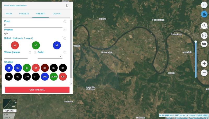
France, a spot near Toulous.

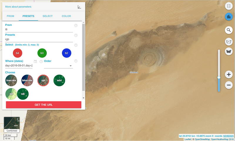
The Sahara desert.

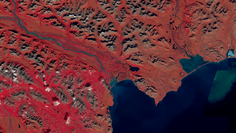
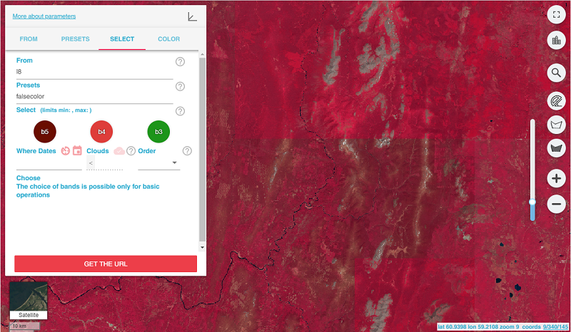
False Colour images 

5, 4, 3 – Traditional Colour Infrared (CIR) Image

Band 5 is Near Infrared (NIR) – this part of the spectrum is one of the most frequently used as healthy plants reflect it mostly: water in their leaves scatters the wavelengths back into the sky. This information gets useful for vegetation analysis. By matching this band with others, one can get indexes like NDVI, which provide more precise measurement of plant condition comparing with only looking at visible greenness.

Pay your attention on how healthier vegetation beams in red more clearly. This band combination is often used for remote sensing of agricultural, forest and wetlands.

Let’s look at image #1 in the 5-4-3 band combination.

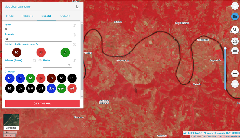
Compare the image made in essential RGB colors: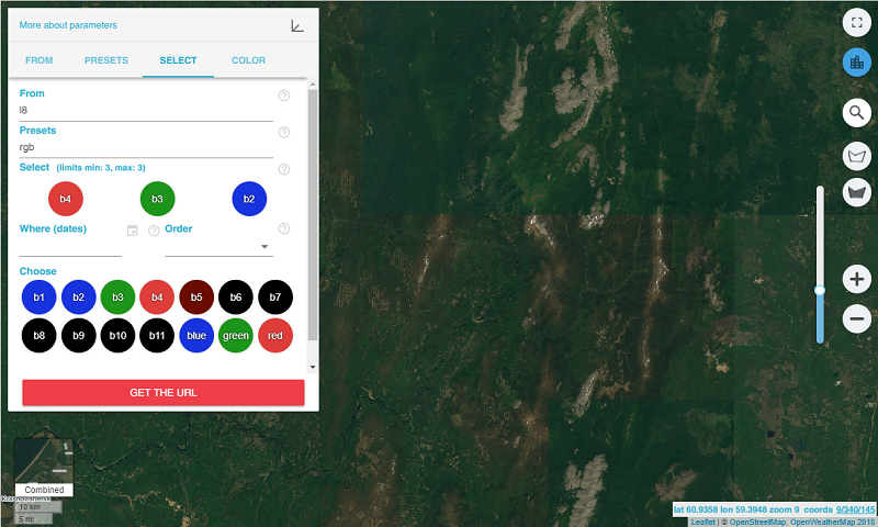

And here is the 5-4-3 band combination:

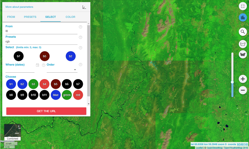
7, 5, 2 – False colour image

This band combination is convenient for the monitoring of agricultural crops which are displayed in bright green colour. Bare earth is showed in purple colour while not cultivated vegetation appears in subtle green.    

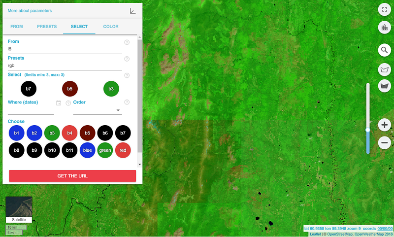
7, 5, 3 – False color image 

This false-color image shows land in orange and green colours, ice is depicted in beaming purple, and water appears to be blue. This band combination is similar to the 7-5-2 band combination, but the former shows vegetation in more bright shades of green.     

 

Image Classification

The goal of classification is to assign each cell in the study area to a known class (supervised classification) or to a cluster (unsupervised classification).

In both cases, the input to classification is a signature file containing the multivariate statistics of each class or cluster.

The result of classification is a map that partitions the study area into classes. Classifying locations into naturally occurring classes corresponding to clusters is also referred to as stratification.

Iso Cluster Unsupervised Classification (Spatial Analyst)

In an unsupervised classification, you divide the study area into a specified number of statistical clusters. These clusters are then interpreted into meaningful classes.

Performs unsupervised classification on a series of input raster bands using the Iso Cluster and Maximum Likelihood Classification tools.

Practical – Unsupervised classifications

Unsupervised classification is done in two stages as follows:

1. Creating Iso-cluster
2. Creating Maximum likelihood classification

1. Steps for Iso-cluster

1. Add data – Composite image
2. Spatial Analysis Tool
3. Multivariate
4. Iso-cluster
5. Input raster bands
6. Check output location
7. Number of classes
8. Ok

1. Steps for Creating Maximum likelihood classification

1. Spatial Analysis Tool
2. Multivariate
3. Maximum likelihood classification
4. Input raster bands
5. Input signature file
6. Output classified Raster
7. Ok

Land use Map

Land use map shows the types and intensities of different land uses in a particular area. For land use map the image classified in last exercise may be used as follows:

Create land use map with classified raster image created in last exercise

This exercise comprises 2 steps

First step

1. Right click on classified image
2. Property
3. Symbology
4. Double click on colored box
5. Change land use type
6. Apply
7. OK

Second step

1. Click layout view
2. Use tools to set map at right place
3. Give title
4. legend (set Item)
5. Scale bar (Set Properties)
6. File – Export – Save

https://www.youtube.com/watch?v=XHOmBV4js_Ehttps://www.youtube.com/watch?v=ilBRHCcM6-Y&t=600s

CHAPTER 5 – GPS & Remote Sensing

Introduction

The Global Positioning System (GPS), originally NAVSTAR GPS, is a satellite-based radionavigation system owned by the United States government and operated by the United States Air Force. It is a global navigation satellite system (GNSS) that provides geolocation and time information to a GPS receiver anywhere on or near the Earth where there is an unobstructed line of sight to four or more GPS satellites.
Obstacles such as mountains and buildings block the relatively weak GPS Signals.
A visual example of a 24 satellite GPS constellation in motion with the Earth rotating. Notice how the number of satellites in view from a given point on the Earth’s surface changes with time. The point in this example is in Golden, Colorado, USA (39.7469° N, 105.2108° W).

Applications

Many civilian applications use one or more of GPS’s three basic components: absolute location, relative movement, and time transfer.

Astronomy: both positional and clock synchronization data is used in astrometry and celestial mechanics. GPS is also used in both amateur astronomy with small telescopes as well as by professional observatories for finding extrasolar planets.
Automated vehicle: applying location and routes for cars and trucks to function without a human driver.
Cartography: both civilian and military cartographers use GPS extensively.
Cellular telephony: clock synchronization enables time transfer, which is critical for synchronizing its spreading codes with other base stations to facilitate inter-cell handoff and support hybrid GPS/cellular position detection for mobile emergency calls and other applications. The first handsets with integrated GPS launched in the late 1990s. The U.S. Federal Communications Commission (FCC) mandated the feature in either the handset or in the towers (for use in triangulation) in 2002 so emergency services could locate 911 callers. Third-party software developers later gained access to GPS APIs from Nextel upon launch, followed by Sprint in 2006, and Verizon soon thereafter.
Clock synchronization: the accuracy of GPS time signals (±10 ns)[94] is second only to the atomic clocks they are based on, and is used in applications such as GPS disciplined oscillators.
Disaster relief/emergency services: many emergency services depend upon GPS for location and timing capabilities.
GPS-equipped radiosondes and dropsondes: measure and calculate the atmospheric pressure, wind speed and direction up to 27 km (89,000 ft) from the Earth’s surface.
Fleet tracking: used to identify, locate and maintain contact reports with one or more fleet vehicles in real-time.
Geofencing: vehicle tracking systems, person tracking systems, and pet tracking systems use GPS to locate devices that are attached to or carried by a person, vehicle, or pet. The application can provide continuous tracking and send notifications if the target leaves a designated (or “fenced-in”) area.[96]
Geotagging: applies location coordinates to digital objects such as photographs (in Exif data) and other documents for purposes such as creating map overlays with devices like Nikon GP-1
GPS aircraft tracking
GPS for mining: the use of RTK GPS has significantly improved several mining operations such as drilling, shoveling, vehicle tracking, and surveying. RTK GPS provides centimeter-level positioning accuracy.
GPS data mining: It is possible to aggregate GPS data from multiple users to understand movement patterns, common trajectories and interesting locations.[
GPS tours: location determines what content to display; for instance, information about an approaching point of interest.
Navigation: navigators value digitally precise velocity and orientation measurements.
Phasor measurements: GPS enables highly accurate timestamping of power system measurements, making it possible to compute phasors.
Recreation: for example, Geocaching, Geodashing, GPS drawing, waymarking, and other kinds of location based mobile games.
Robotics: self-navigating, autonomous robots using a GPS sensors, which calculate latitude, longitude, time, speed, and heading.
Sport: used in football and rugby for the control and analysis of the training load.[98]
Surveying: surveyors use absolute locations to make maps and determine property boundaries.
Tectonics: GPS enables direct fault motion measurement of earthquakes. Between earthquakes GPS can be used to measure crustal motion and deformation to estimate seismic strain buildup for creating seismic hazard maps.
Telematics: GPS technology integrated with computers and mobile communications technology in automotive navigation systems.